Statistics that Measure Central Tendency
Mean
Your have
probably used the
mean since elementary school. There it is was called the
average. The mean
(or average) of a collection of numbers is
computed by adding the numbers and dividing by the number of
numbers. For example the mean of the numbers 2,3,3,4,5,6
is 23/6=3.8 rounded to the nearest tenth. In formula
form, the mean of n numbers, x1, x2,
..., xn is given by the sum of the numbers (x's)
divided by n, the number of numbers, or

For a data set presented as numbers
together with the frequency of occurrence of each number, as
in the next table, the computation of the mean is slightly
modified.
| Number |
Frequency |
| 2 |
2 |
| 3 |
6 |
| 4 |
7 |
| 5 |
3 |
| 7 |
3 |
| 9 |
2 |
Add another column consisting of each
number multiplied by the frequency of occurrence of that
number to the table. Then find the sum of this column as shown:
|
Number |
Frequency |
Number*Frequency |
| 2 |
2 |
4 |
| 3 |
6 |
18 |
| 4 |
7 |
28 |
| 5 |
3 |
15 |
| 7 |
3 |
21 |
| 9 |
2 |
18 |
| Sum
of (Numbers*Frequencies)= |
104 |
The mean is the (Sum of
Numbers*Frequencies)/(Sum of Frequencies). In the
example the sum of the frequencies is 23, so the mean is
104/23=4.5. In formula form, the mean of numbers x which
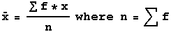
occur with frequency f is given by
The mean is easy to compute, and as
mentioned above, you have
probably used it before, but it has one major drawback--an extremely
large or small number will cause a larger than desired
change in the mean. For example the mean of
2,3,4,5, and 6 is 4. However, if another number, say 20, is added to the set, the mean of the new
set of numbers, 2,3,4,5,6, and 20 is now 40/6=6.7.
Certainly the mean should increase but increasing from 4 to
6.7 might be considered to be too much of a change.
In presenting housing prices in the newspaper the mean price of a
home is usually not used, simply
because the mean is made too high by the relatively few expensive
homes in a typical community. Median home prices are
used instead of mean home prices. The
next section discusses the median.
At the bottom of this page is a link
to the FOCUS dataset. Open it and under the STAT
menu you will find a choice called Summary
Stats. Use that to find the mean of each of
variable in the FOCUS dataset. Other descriptive statistics introduced below are also
computed for each of the variables. Make a
histogram of each variable and see how the descriptive
statistics relate to the shape of the histogram.
Also, you can verify the example computations in these
notes by opening Webstat--push the orange button at
the bottom of this page, select the Clear Data
choice under the Data menu, and type the numbers for
which you want the mean or other statistics into
a column. Once you have the numbers in a column, you
can make any of the Webstat graphs and compute any
numerical statistics on your numbers by selecting
Histogram under the Graphs menu and Summary Stats
under the Stats menu.
Median
The
median of a collection of numbers is, in a certain sense, the
'middle' number of that set. For example the median of
the numbers 2,3,4,5,8 is 4 because 4 is the 'middle' number.
The numbers 2,3,4,5,8,10 don't have a single middle
value. What is the median of them? It is
defined as the average of
the two middle numbers, 4 and 5. The median is then
(4+5)/2=4.5.
The process for computing the median
of a set of n numbers is:
-
Sort the numbers and arrange them from
smallest to largest.
-
Consider the smallest number to be in position 1, the next number in the sorted list
to be in position 2, the next in position 3, etc.
-
The median will be the number in
position (n+1)/2. If (n+1)/2 is a whole number,
the median will be the number lying in that position.
If (n+1)/2 is a fraction, say 7.5, the median will be
the average of the two numbers in positions 7 and 8.
Example: Find the median of the numbers
2,3,1,4,4,5,7,2,3, and 8.
-
In sorted order the numbers are
1,2,2,3,3,4,4,5,7,8
-
The numbers with their positions are
| Position |
1 |
2 |
3 |
4 |
5 |
6 |
7 |
8 |
9 |
10 |
| Number |
1 |
2 |
2 |
3 |
3 |
4 |
4 |
5 |
7 |
8 |
-
The median is the number in position
(10+1)/2=5.5. Since 5.5 is not a whole number, the
median is the average of the numbers in positions 5 and
6, or the average of 3 and 4 which equals 3.5. The
median is 3.5.
Mode
The
mode is the number that occurs most frequently. For the
set of numbers 2,3,4,5,5,6, the mode is 5. The set of
numbers 2,3,4,5,5,6,6 has two modes, 5 and 6. It is
bimodal. However, when all numbers in a set occur with
the same frequency, the set of numbers has no mode. For
example, the numbers 2,2,3,3,4,4,5,5 have no mode.
Quartiles and Percentiles
The
median divides a set of numbers into halves. Quartiles
divide a set of numbers into quarters and percentiles divide a
set of numbers into hundredths. You may taken achievement tests
in school and received your result in the form of a percentile
score.
If you were told that you were at the 92nd percentile, then
92% of the test scores were equal to or lower than your score and
8% of the test scores were equal to or higher than your score.
There are three quartiles for a set of
numbers, the 1st quartile, denoted by Q1, the 2nd quartile
denoted by Q2, and the 3rd quartile denoted by Q3. The
2nd quartile is also usually called the median, and you have seen how
to compute it. The quartiles divide the dataset
into quarters. To compute the 1st quartile, Q1, simply find
the median of all numbers in the dataset that are less than or
equal to the median. To compute the 3rd quartile, Q3,
find the median of all numbers in the dataset that are greater
than or equal to the median.
| Position |
1 |
2 |
3 |
4 |
5 |
6 |
7 |
8 |
9 |
10 |
| Number |
1 |
2 |
2 |
3 |
3 |
4 |
4 |
5 |
7 |
8 |
The median of the numbers in the table just
above was found to be the average of the numbers in positions 5 and
6, that is (3+4)/2=3.5. Then the 1st quartile is the
median of the numbers that are less than or equal to 3.5, that
is the median of 1,2,2,3,3. These numbers are sorted and
the positions are the same as in the last table. Since
there are 5 numbers, the median is the
number in position (5+1)/2=3, and this number is 2. Q1=2. The
3rd quartile is the median of the numbers greater than or
equal to 3.5, or the median of 4,4,5,7,8. Again, since
there are 5 numbers here, the median of this set of 5 numbers
is the number in position 3, that is 5. Q3=5.
Resources
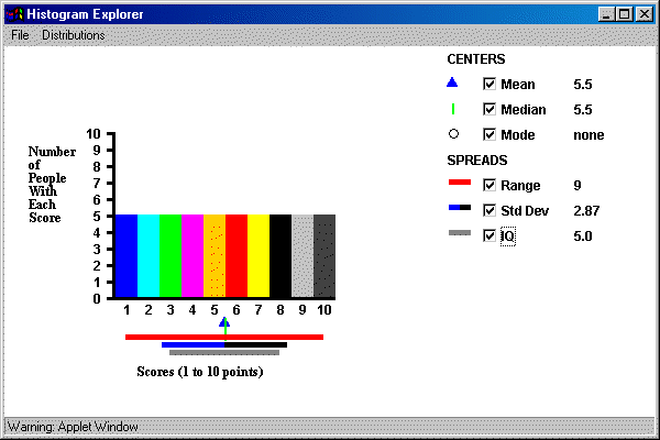
A demonstration page for descriptive statistics showing the relationship
between the histogram of a set of numbers and the corresponding descriptive statistics is
found by following this link
to a page designed by Eric Scheide. The following display shows the
page.
Statistics that Measure Variability
Range
The
range of a set of numbers equals the largest number minus the
smallest number. The range of the numbers 3,5,9,9,10,13
is 13-3=10. Like the mean, range had the disadvantage of
changing by too much when an extremely large or small
value is added to a dataset. The next statistic, the interquartile range
does not have this drawback.
Interquartile Range (IQR)
The
interquartile range is the third quartile minus the first
quartile, IQR=Q3-Q1. For the set of numbers
1,2,2,3,3,4,4,5,6,7, in the examples above Q1 was found to be
2 and Q3 was found to be 5. Thus the interquartile range
is 5-2=3. Compare this with the range=7-1=6.
Standard Deviation
The measure of variability used most often
is called the standard
deviation. The standard deviation is roughly the average
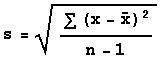
of squared deviations from the mean. The formula for
the standard deviation of x1, x2,
...,xn is
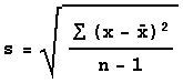
where x-bar is the mean of the numbers.
As an example consider the numbers
2,3,4,5,6. The mean is 4. Then the differences
between each of the numbers and the mean are (2-4)=-2,
(3-4)=-1, (4-4)=0, (5-4)=1, and (6-4)=2, respectively.
The formula indicates that these numbers must be squared and
added. The squares are 4,1,0,1, and 4, and the sum is
10. Finally the formula directs you to divide this sum
by the number of numbers-1, i.e. n-1, and take the square
root. This results in the square root of 10/4 or the
square root of 2.5 which is approximately 1.58.
The square of the standard deviation is
called the variance of the set of numbers. The
variance has the drawback that the units of standard
deviation are the square of the units of the numbers used to
compute variance. For example, if the units of the
numbers shown in the last example are inches, the units of
the variance are square inches.
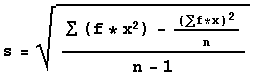
An easier formula for computing the standard
deviation is
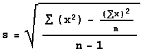
and the easy formula for computing standard deviation for
numbers, x, given along with frequencies, f, is
Other Statistics and Displays
Boxplots (Also called Box and Dot or Box and
Whisker Plots)
A boxplot displays the center (as
given by the median) of a dataset, the range, and the
quartiles. The next picture shows two boxplots,
one of the SAT Verbal and the other the SAT Math
scores from the FOCUS dataset.
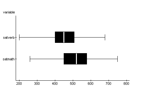
The white line in the box lies above
the median value for that variable. You can see
that the median SAT Verbal score is around 460 and the
median SAT Math score is about 540. The left
side of the box lies above the 1st quartile and the
right side of the box is positioned above the 3rd
quartile of the variable. So for SAT Math the
first quartile is about 460 while the third quartile
is approximately 590. Since 25% of the data
values are less than the first quartile and 25% of the
data values are greater than the third quartile, the
boxes indicate the range of values in which the middle
50% of the numbers lie. From the above graph you
can see that the middle 50% of the SAT Math values are
more spread out than the middle 50% of SAT Verbal
scores. The horizontal line from the right of
each box stops where the short vertical line
positioned above the largest number for that variable,
and the horizontal line from the left of each box
stops at the short vertical line over the smallest
value for the variable. The distance from the
smallest value to the largest value, the range is
shown in the graph.
The boxplot displays variability,
center, and shape of a dataset. In the above
graph of SAT Math and Verbal scores, you can see that
both variable have approximately the same amount of
variability, the center of the SAT Math scores is
greater than the center of the verbal scores, and both
of the variables have an approximately symmetric
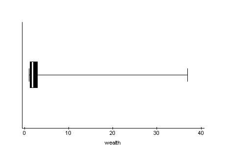
shape. The next boxplot of the billionaires92
wealth variable shows a dataset that is strongly
skewed to the right. Even the position of the
median within the box shows a right skew for the
middle 50% of the wealth data.
What is the relationship between the
histogram and the boxplot of a set of numbers?
To experiment with histograms and the corresponding
boxplots open this link.
When the link opens select Relative Frequency in the
left dropdown menu and Boxplot from the right dropdown
menu. Then, by pointing at the axis with your
mouse cursor and clicking, you can add numbers.
The vertical red bars show the histogram of the
numbers that you have added and the horizontal red
display below the histogram shows the boxplot that
goes with the histogram. Try various shaped
histograms and see how the boxplot corresponds with
the histogram.
Standard Scores
Suppose you and a friend are both taking
Statistics 1 but are in different sections. You both take a
midterm examination and wish to compare your performances on the
exam. You received a score of 80 in a section that had a
mean of 76 and a standard deviation of 5, while your friend
received a score of 76 in a section that had a mean of 66 and a
standard deviation of 8. Who performed better? In
order to determine this, the scores need to be placed on the same
footing, that is be modified as if they both came from a test with
the same mean and standard deviation. This can be done by
subtracting the mean of the section and dividing by the standard
deviation of the section. That is (x-mean)/(standard
deviation) is computed for each score. For your score
of 80 this results in (80-76)/5=0.8 while for your friend's score you
get (76-66)/8=1.25. This means that your friend had a better
performance.
The standard score corresponding to a number x, denoted by z,
is given by the next formula:

where x is the actual score, x-bar is the mean of the set of numbers,
and s is the standard
deviation of the numbers. The standard score indicates how
many standard deviations above (if z is positive) or below the
mean (if z is negative) the number, x, falls.
Sample
and Population Statistics
All
of the statistics used above apply to samples--they are
called sample statistics. The related statistics
for populations are slightly different. The
following notations and differences in formulas apply:
Descriptive measures for a
population are called parameters of the population
while related measures for a sample are called
statistics of the sample. -
The size of a sample is usually
denoted by n while the size of the population is
given by N
-
The sample mean is written as
x-bar while the population mean is usually denoted
by µ.
-
The sample standard deviation is
called s and the population standard deviation is
called sigma.
-
The formula for sample standard
deviation is
but the formula for population
standard deviation is
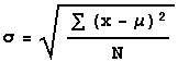
There are two differences.
First, the sample mean is replaced by the
population mean. This isn't surprising.
The second difference, the divisor for the population standard deviation
is N, while the divisor for the sample standard deviation is
n-1 is harder to explain. There is a
good statistical reason for the difference but
that reason will be left to another statistics
course. You should simply use the formula
that is
appropriate for the situation. If you are
told that you have a population, use the second
formula, and for a sample use the first formula.
An easier-to-use formula for population standard
deviation is
If the numbers are given along
with frequencies the formula to use is
where N is the sum of the
frequencies.
Resources
See Section 3.5 in the Weiss textbook.
To work with the entire Focus Database
from within WebStat use the next link.
|
|
|
|