Hypothesis Testing 2--Testing for Population Means
|
In Hypothesis Testing 1, you were introduced to the ideas of hypothesis
testing in the context of deciding whether a coin was fair or biased in favor of
heads. In this section hypothesis testing concerning population means is
explored.
 |
Testing H0: µ=µ0 vs. Ha: µ>µ0 When the
Population Standard Deviation is Known
 |
Assumptions
 | A random sample of size n is taken from some population. Either
the population is normal in which case n can be of any size, or the population
distribution is unknown in which case n should be 30 or more. In the following
examples suppose n=36.
|
 | The standard deviation, sigma, of the population is known. In the
examples suppose sigma=5.
|
 | The level of significance, alpha, is given. In the following
examples suppose alpha=0.05.
|
In all three methods it is assumed that the distribution of sample means
for samples of size n is, at least, approximately normal with mean given by µ0 (assume
that µ0 is 50 for the next examples) from the null hypothesis, and standard deviation
sigma/Sqrt[n] (which equals 5/Sqrt[36]=5/6).
|
 | Method 1--The Critical xbar Method:
 | Step 1: Based on the null and alternative hypotheses and given
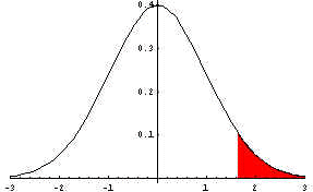
alpha, find a critical z-value (or z-values). Remember
that alpha is the tail probability (in the right tail for the given alternative
hypothesis). For alpha=0.05, the critical z-value is 1.645. This
is the
z-value below the vertical line that defines the left side of the red-shaded area.
The red-shaded area has probability 0.05.
|
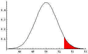
 | Step 2: Now use the equation  with z=1.645,
µ=50 from the null hypothesis, sigma=5, and the square root
of n=6 to solve for xbar. This solution is called the critical xbar value,
or more simply, the critical value.. It equals 51.3708. If the actual sample mean of the random sample of
size 36 is 51.3708 or greater, you reject the null hypothesis. The rejection region
is shown in red in the next graph. with z=1.645,
µ=50 from the null hypothesis, sigma=5, and the square root
of n=6 to solve for xbar. This solution is called the critical xbar value,
or more simply, the critical value.. It equals 51.3708. If the actual sample mean of the random sample of
size 36 is 51.3708 or greater, you reject the null hypothesis. The rejection region
is shown in red in the next graph.
|
 | Step 3: Take the random sample of size n and compute xbar, the
sample mean. Compare this with the critical value to either
accept or reject the null hypothesis.
|
|
 | Method 2--The Critical Z Method:
 | Step 1: Based on alpha and the alternative hypothesis, find a critical z-value
or z-values (1.645 for the example).
|
 | Step 2: Take the random sample and compute the sample mean, xbar
(for
example, suppose the sample xbar that you get is 52.3).
|
 | Step 3: Put xbar along with mu, sigma, and n into  .
The resulting z-value is called the computed z-value. (For the example, the
computed z-value is 2.76). If the computed z-value lies outside of the critical
z-value found in 1, reject the null hypothesis; otherwise, fail to reject the null
hypothesis. (For the example, 2.76 lies outside of 1.645, so you would reject the
null hypothesis) .
The resulting z-value is called the computed z-value. (For the example, the
computed z-value is 2.76). If the computed z-value lies outside of the critical
z-value found in 1, reject the null hypothesis; otherwise, fail to reject the null
hypothesis. (For the example, 2.76 lies outside of 1.645, so you would reject the
null hypothesis)
|
|
 | Method 3--The p-value Method:
 | Step 1: Take a random sample and compute the sample mean, xbar. (Suppose,
for
example, that xbar is 52.3)
|
 | Step 2: Put the computed xbar along with mu, sigma, and n into  . (For the example the computed z-value is 2.76) Find the
probability in the tail beyond (beyond is determined by the alternative hypothesis) the
computed z-value. If the test is a 1-tail test, this probability is called the p-value. (For the example the
p-value=0.003). If the test is a 2-tail test, double the probability to
find the p-value. . (For the example the computed z-value is 2.76) Find the
probability in the tail beyond (beyond is determined by the alternative hypothesis) the
computed z-value. If the test is a 1-tail test, this probability is called the p-value. (For the example the
p-value=0.003). If the test is a 2-tail test, double the probability to
find the p-value.
|
 | Step 3: If the p-value is less than or equal to alpha, reject the null
hypothesis. If the p-value is greater than alpha, fail to reject the null
hypothesis. (For the example, since 0.003<0.05, you would reject the null
hypothesis)
|
|
|
 | Type I and Type II Errors
To review, a Type I error occurs when the null hypothesis is true but the
test rejects it, while a Type II error occurs when the null hypothesis is
false but the hypothesis test accepts it. P[Type I error]=Alpha and
P[Type II error]=Beta. In the next examples Type I and Type II errors
will be calculated in hypothesis tests for a population mean.
In all the following examples assume that a random sample of size 36 has
been taken from a population with standard deviation 5. Assume that
the sample mean for this sample of size 36 is xbar=52.7. Finally,
assume that the significance level, alpha, is 0.05.
 |
Example 1: Testing H0: µ=50 vs. Ha: µ>50
Using the critical xbar method, the critical z-value is 1.645.
From the equation  you
you
get 1.645=(critical xbar-50)/(5/6), and solving this for the critical
xbar results in critical xbar=51.37. Since the sample xbar is
52.7, you would reject the null hypothesis in favor of the alternative.
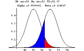
What is beta, the probability of a Type II error if the population mean
is in fact 52? The computation is not shown here but in the title
section of the next
graph
you see that beta is 0.22.
|
 | Example 2: Testing H0: µ=50 vs. Ha: µ<50
This example mirrors example 1. Again, using the critical xbar method, the critical z-value is
-1.645.
From the equation  you get -1.645=(critical xbar-50)/(5/6), and solving this for the critical
xbar results in critical xbar=48.63. Since the sample xbar is
52.7, you would accept the null hypothesis.
What is beta, the probability of a Type II error if the population mean
is in fact 52? The computation is not shown but beta is equal to
0.99.
|
 | Example 3: Testing H0: µ=50 vs. Ha: µ<>50 (<>
means not equal)
In Example 3, you the alternative hypothesis leads you to reject the
null hypothesis for either large or small values of xbar. This is
a two tail test. There are two critical z-values, -1.96 and +1.96.
From the equation  you
get -1.96=(critical xbar-50)/(5/6), and +1.96=(critical xbar-50)/(5/6).
Solving these two equations results in the critical
xbar values of 48.37 and 51.63. Since the sample xbar is
52.7, you would reject the null hypothesis.
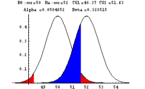
What is beta, the probability of a Type II error if the population mean
is in fact 52? The computation is again not but from the title
section of the next
graph you see that beta is 0.33. The red shaded area is alpha, the
probability of a Type I error, and the blue shading is beta, the
probability of a Type II error.
|
|
 | Testing H0: µ=µ0 vs. Ha: µ>µ0 When the
Population Standard Deviation is Unknown
In finding confidence intervals for the population mean, for small
samples from a normally distributed population where the population standard
deviation was unknown, you had to use Student's t-distribution to complete
the solution. The situation is the same in hypothesis testing.
Instead of using  , you must use
  where the expression has a t-distribution with n-1 degrees of freedom.
 |
Example: A random sample taken from a normal population produced the
numbers 8, 10, 9, and 8.6. At the 5% significance level, is the
population mean equal to 10?
First, the null and alternative hypotheses must be stated. They
are
H0: µ=10 and Ha: µ<>10 where '<>' means
not equal.
Since the statement of the example
expresses no preference in determining whether the mean of the population is
less than or greater than 10, the 'not equal' alternative hypothesis is
used. The p-value approach using the t-statistic shown above is
employed.
From the random sample
values, you find xbar=8.9 and s=0.84.
Substituting them into the
t-statistic formula, you get calculated t=(8.9-10)/(0.84/Sqrt(4))=(-1.1)/(0.84/2)=-2.62.
Since a two
tail test is indicated by the alternative hypothesis, the p-value is
found by computing the area under Student's t-distribution with 3
degrees of freedom to the left of -2.62 and doubling the result. Student's t-distribution is symmetric about zero,
so instead of
finding the area to the left of -2.62, you can find the area to the
right of 2.62. In the row of the 't-table' corresponding to 3
degrees of freedom, you find 2.353 and 3.182. The number that you
seek, 2.62 lies between these two numbers. Then the area under the
Student's t-distribution with 3 degrees of freedom to the right of 2.62
must lie between 0.025 and 0.05, the numbers at the top of the columns
corresponding to 2.353 and 3.182. The p-value lies between
2*0.025=0.05 and 2*0.05=0.10.
The p-value is larger than 0.05 so the null hypothesis is accepted.
|
|
|

 with z=1.645,
µ=50 from the null hypothesis, sigma=5, and the square root
of n=6 to solve for xbar. This solution is called the critical xbar value,
or more simply, the critical value.. It equals 51.3708. If the actual sample mean of the random sample of
size 36 is 51.3708 or greater, you reject the null hypothesis. The rejection region
is shown in red in the next graph.


 where the expression has a t-distribution with n-1 degrees of freedom.