Continuous Random Variables
Some differences between discrete and continuous probability distributions:
| Discrete Random Variables | Continuous Random Variables |
|---|---|
| Density functions are nonnegative for all real numbers but greater than zero only at a finite or countably infinite number of points. | Density functions are nonnegative for all real numbers and are greater than zero on certain intervals of real numbers. |
| The sum of the discrete density function summed over all real numbers is 1. | The integral of the continuous density function integrated over all real numbers is 1. |
| They may have nonzero probability at some real numbers. | They have zero probability at every real number. |
| The probability of an event is found by summing the values of the discrete pdf at real numbers defined by event. | The probability of an event is found by integrating the continuous pdf for all real numbers defined by the event. |
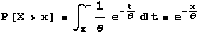
The next statement shows how to compute the probability that continuous random variable X with pdf f(x) lies in the interval [a,b].
![]()
The cumulative density function (cdf) for random variable X with pdf f(x) is defined as follows:
![]()
Some of the commonly used continuous random variables are introduced below. Continuous random variables are introduced by giving either their pdf or cdf.
In dealing with continuous random variables, you may find the resources for graphing and integrating functions on the Mathematical Toolkit page at Vanderbilt University helpful.
To Top
The expected or average value of random variable X with pdf f(x) is given by
![]()
and the expected value of the function g(X) of X is computed as
![]()
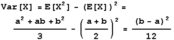
By taking g(x) = x2, in the last formula you can find E[X2], and use it in the formula Var[X]=E[X2]-(E[X]2) to find the variance of the random variable X.
To Top
-
Uniform Random Variable with Parameters a and b
-
Definition
A Uniform Random Variable with parameters a and b is a continuous random variable that can assume values in any small subinterval of length d within the interval from a to b with equal probability. The probability is proportional to the length, d, of the interval.
-
Simulation
Assume that a continuous uniformly distributed random variable, R, on [0,1] can be generated by the computer. The Uniform RV with parameters a and b can then be simulated by having a computer generate a value of a random variable, R. Call the value generated r. Then the value of the uniform random variable, X, with parameters a and b is a + r (b-a).
A Uniform RV with parameters a and b can also be simulated by a spinner that has values numbered from a to b.
-
Probability Distribution (pdf) and Cumulative Distribution Function (cdf)
The pdf is denoted by f(x) and the cdf is denoted by F(x).

It is easy to see that f(x) defines a probability density function because it is nonnegative and the integral of the function from -infinity to infinity is 1.
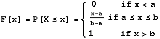
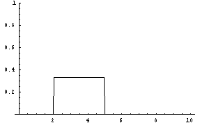
The next two graphs show the pdf (left graph) and cdf (right graph) of a uniform random variable with parameters 2 and 5.
-
Mean and Variance
-
Mean

-
Variance
Var[X]=E[X2]-(E[X]2. First E[X2] is found:
Now the formula shown above is applied to find the variance:
-
-
To Top
-
Exponential Random Variable with Parameter theta (
 >0)
>0)-
Definition
The exponential random variable with parameter theta often gives the waiting time between events. For example, if customers arrive at a service point according to a Poisson distribution, the time between arrivals has an exponential distribution. The exponential random variable is also used to model the service time used in servicing customers. For example, the time needed for a computer to complete a job may be exponentially distributed.
By following this link you can reach a web page that has more information on exponential random variables and by pressing the red die in front of exercise 5, you can see and modify graphs of exponential random variables. In this simulation, the form of the exponential is re-rx for x>0 instead of the form shown below.
-
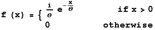
Probability Distribution (pdf) and Cumulative Distribution Function (cdf)
The pdf and cdf for an exponential with parameter theta are shown next. The pdf is denoted by f(x) and the cdf is denoted by F(x).

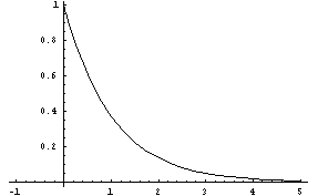
Graphs of the pdf (left) and cdf (right) for an exponential RV with parameter 1 are shown next.
-
Simulation
Simulation of a continuous random variable, X, can be carried out by finding the inverse of the cumulative distribution function (cdf) for X. A result that will not be justified here says that if X has cdf F with inverse function F-1, then random variable X can be simulated by generating values of a continuous uniform random variable R on [0,1] and finding F-1[R]. The values F-1[R] provide a simulated values of X. This method is limited to continuous random variables for which a closed-form expression for F-1 can be found.
In the case of the exponential F-1[R] = theta(-ln(1-R)).
Follow this link to a simulation of the Exponential Random Variable. Push the red die in front of exercise 5 to run the simulation. Note that in this simulation, the form of the exponential is re-rx for x>0 instead of the form shown above.
-
Mean and Variance
-
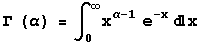
Gamma Function
The gamma function is defined by the following improper integral.
This integral has the property that
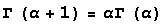
and this can be used to show that for any positive integer, n,

By making the substitution x =
 y
and dx = dy
in the first integral of the following display, you get the identity
shown next.
y
and dx = dy
in the first integral of the following display, you get the identity
shown next.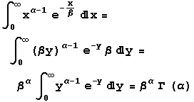
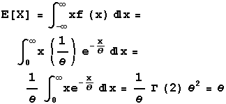
These gamma function identities are used to find the mean and variance of the exponential distribution
-
Mean
-
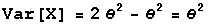
Variance
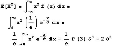
But Var[X]=E[X2]-(E[X]2) so
-
-
To Top
-
Normal Random Variable with Parameters mu (
 ) and sigma (
  )
)-
Definition and Simulation
The Normal Random Variable is defined by the probability density function shown in the next section. As you will see the normal random variable has a 'bell-shaped' pdf. This 'bell-shaped' density function is centered at the mean
and has variability given by standard deviation .As you will see in the next chapter, a reason that the Normal RV arises in so many situations can be stated simply as 'averages are approximately normally distributed.' This statement provides a means of simulating a normal random variable: find averages of randomly selected numbers--these averages will have an approximate normal distribution.
Follow this link to a simulation of a normal random variable. Press the red die in front or exercise 4.
-
Probability Distribution (pdf) and Cumulative Distribution Function (cdf)
The formula for the pdf is shown next.
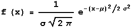
In the normal pdf x can be any real number.
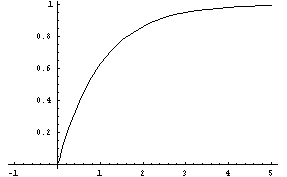
The cdf for the normal distribution has no closed-form expression. It can be expressed as the integral of the pdf from -infinity to x. There are tables of the cdf (see the back of your textbook) for the special case
=0
and =1.
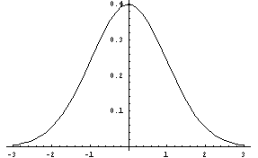
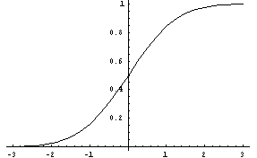
This special case RV is called the Standard Normal Random Variable.
Once you know the cdf for the standard normal RV, you can find the
probabilities for any other normal RV by using a z-score formula.
The next display shows the pdf (left graph) and cdf (right graph)
for the Standard Normal RV.
-
Mean and Variance
The mean and variance computations are shown for the Standard Normal RV. This special normal random variable is denoted by Z.
-
Mean
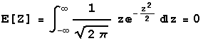
This integral is zero because the function is an odd function.
-
Variance
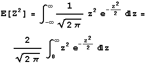
The integral identity follows because the function being integrated is an even function. Make the change of variable u = z2 so du = 2zdz. The last integral above then becomes
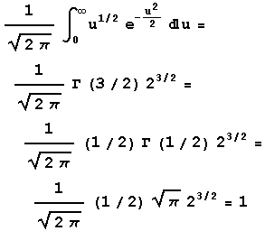
The last line follows because the gamma function evaluated at 1/2 is the square root of pi.
Since the mean of the Standard Normal RV is 0, Var[Z] = E[Z2]-(E[Z]2) = 1-0 = 1.
-
-