4. Discrete Rand. Vars.
[ Home ] [ Up ]

Discrete Random Variables

• Definition and Probability Distributions

  • A random variable is a real-valued function defined on the sample space of an experiment.  A discrete random variable can only take on a finite or countably infinite number of values.

    • Example 1: A coin is flipped.  Random variable X takes the value 1 if the coin lands heads, and X takes the value 0 if the coin shows tails.
      
      

    • Example 2: Three balls are drawn without replacement from a container that holds 80 balls, 20 of the balls are green and 60 are white.  Random variable G is a count of the number of green balls drawn.
      
      

    • Example 3: A fair coin is tossed 3 times.  Random variable S is the total number of heads in the three tosses.
      
      

  • Given a random variable, X, and real number, x, p(x) = P[X=x] is the probability that X takes the value x.  For a discrete random variable, 

  P[X=x] is nonnegative

  and

   

  The collection of pairs, (x,p(x)), for all real x is the probability distribution (also called the probability density function or pdf) of X

  • Probability distributions (or pdf's) for the Random Variable Examples.

    A Java applet that shows graphs of probability distributions can be found at this link.

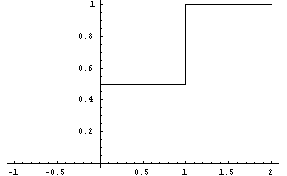
    • Example 1:  The probability distribution of X is given by P[X=0]=P[X=1]=1/2 and P[X=k]=0 for all other numbers k.  Notice that the sum of probabilities is 1.
      
      

    • Example 2: The probability distribution of X is given by for g=0, 1, 2, or 3, and P[G=g]=0 for all other real numbers, g.  By computing the combinatorial coefficients for g=0, 1, 2, and 3, you can verify that P[G=0]+P[G=1]+P[G=2]+P[G=3]=1 as required by the second property of a probability distribution.  Follow this link to see a graph of the probability distribution of this random variable.  When you reach the page go to exercise 4 and press the red die.  This will open a Java applet.  When this opens set N=80, R=20, and n=3.  The graph of the probability distribution will be displayed.
      
      

    • Example 3: The probability distribution of S is given by for s=0,1,2,3 and P[S=s]=0 for all other values of s.  Again, the sum of probabilities can be shown to be 1.  Follow this link to see a graph of the probability distribution of this random variable.  When you reach the page go to exercise 4 and press the red die.  This will open a Java applet.  When this opens set and n=3 and leave p at 0.50.  The graph of the probability distribution will be displayed.
      
      

  • The Distribution Function (also called the cumulative distribution function or cdf) of random a random variable, X, is defined by

     for any real number b

  if X is a discrete random variable, this becomes

  

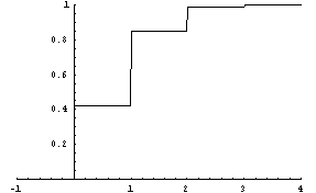
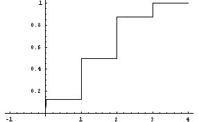
  • The cumulative distribution function is a nondecreasing function (since, at least in the discrete case, it is a sum of nonnegative probabilities) that approaches 1 for large values of x.  For a discrete random variable, the cdf is a step function.
    
    

  • Cumulative Distribution Functions (or cdf's) for Examples

    A Java applet that shows graphs of probability distributions (pdf's) and cumulative distribution functions (cdf's) can be found at this link.

    • Example 1: 
      
      
      
      
      

    • Example 2: 
      
      
      
      
      

    • Example 3:
      
      
      
      

To Top

• Expected Values, Variance, and Standard Deviation

  • The expected value (also called the mean value or simply the mean) of a random variable, denoted by µ=E[X], gives the 'average value' of the random variable.  In the case of a discrete random variable, it is given by

  

  • Expected Values for Random Variable Examples

    • Example 1: E[X] = 0(1/2) + 1(1/2) = 1/2
      
      

    • Example 2: E[G] = 0(0.417) + 1(0.431) + 2(0.139) + 3(0.014) = 0.75
      
      

    • Example 3: E[S] = 0(1/8) + 1(3/8) + 2(3/8) + 3(1/8) = 12/8 = 3/2
      
      

  • The Expected Value of a Function, g(x), of Random Variable X is given by 

   

  • The Variance of a random variable measures variation from the mean of the random variable.  It is found by using the function g(x) = (x-µ)² in the last definition.
    
    
    

    

    
    

    The variance can (and should) be found using the algebraically equivalent formula:

    

    The last statement says that Var[X] = E[X²] - E[X]², in words, the variance of X is the expected value of the square of X minus the square of the expected value of X.

  • Variances for Random Variable Examples

    • Example 1: Var[X] = 0²(1/2) + 1²(1/2) - (1/2)² = (1/2) - (1/4) = 1/4
      

    • Example 2: Var[G] = 0²(0.417) + 1²(0.431) + 2²(0.139) + 3²(0.014) - 0.75² = 0.548
      

    • Example 3: Var[S] = 0²(1/8) + 1²(3/8) + 2²(3/8) + 3²(1/8) - (3/2)² = 3/4
      
      

  • The Standard Deviation of a random variable is the square root of the variance.  It is given by 

    
    
    
    

  • Standard Deviations for Random Variable Examples

    • Example 1: Standard Deviation of X = (1/4)^1/2 = 1/2
      
      

    • Example 2: Standard Deviation of G = (0.548)^1/2 = 0.740
      
      

    • Example 3: Standard Deviation of S = (3/4)^1/2 = 0.866

To Top

• Chebyshev's Theorem: Let X be a random variable with mean µ and standard deviation sigma.  Then 

To Top

• Properties of a Bernoulli Random Variable with Parameter p

  • Definition

  A Bernoulli Random Variable can only assume values 0 or 1.  A value of 0 is usually associated with the failure of an experiment and 1 is associated with the success of the experiment.

  • Simulation

  A Bernoulli RV, X, with parameter p can be simulated by having a computer generate a random number, R, from the interval [0,1].  If R is between 0 and p, set X=1, otherwise set X=0.  
  
  Another way to simulate X is to place uniform pieces of paper in a box--write 1's on proportion p of the pieces and nothing on the remaining pieces.  Draw one piece of paper and let X=1 if the paper has 1 written on it and X=0 if the paper does not have 1 written on it.

  You can find a simulation by pressing the red die in front of Exercise 4 at this link.  

  • Probability Distribution (pdf)

                      p(x) = P[X=x] = p^x(1-p)^1-x for x=0 and 1 
  
                      p(x) = 0 for all other real x.
  
              You will usually see 1-p = q.  Note that the probability distribution sums to 1 since q + p = 1.
  

  • Mean and Variance

    • Mean or Expected Value

                E[X] = 0(1-p) + 1p = p
    

    • Variance

                Var[X] = 0²(1-p) + 1²p - p² = p(1-p) = pq
    
    

• Properties of a Binomial Random Variable with Parameters n and p

  • Definition

  1. An experiment is performed n times.  
  
  2. Each performance of the experiment results in a success, S, or failure, F with P[S] = p and P[F] = 1-p = q.  
  
  3. Each performance of the experiment is independent of all other performances.  
  
  4. The Binomial Random Variable, X, with parameters n and p is the count of successes in the n performances of the experiment. 
  
  

  • Simulation

  A Binomial RV, X, with parameters n and p can be simulated by having a computer generate n random numbers between 0 and 1.  Count the number of these random numbers that lie between 0 and p.  This is the value of X.  
  
  Another way to simulate this random variable is to  place pieces of paper in a box--proportion p of the pieces of paper have 1's written on them, and the other pieces have nothing written on them.  Draw n slips of paper replacing each one before drawing the next.  Let X=number of pieces drawn with 1's on them.

  You can find a simulation by pressing the red die in front of Exercise 4 at this link.  

  • Probability Distribution (pdf)

              p(k) = P[X=k] =_nC_k p^k(1-p)^n-k = _nC_k p^kq^n-k for k=0, 1, 2,...,n 
  
              p(k) = 0 for any other real k.  
  
                    _nC_k = (n!)/(k!(n-k)!) is the number of combinations of n things taken k at a time

  The probabilities sum to 1 because 

  

  by the Binomial Theorem.  Replacing a by p and b by 1-p, the right hand side of the last expression is 1ⁿ = 1.
  
  

  • Mean and Variance

    In finding the mean and variance, consider the relationship between a Bernoulli RV with parameter p and a Binomial RV with parameters n and p.  The Binomial RV can be thought of a the sum of n independent Bernoulli RVs with parameter p.  That is, X = X₁ + X₂ + X₃ + ... + X_n where X_i is a Bernoulli RV with parameter p that equals 1 if the ith performance of the experiment results in a success and X_i is 0 if the ith performance of the experiment results in a failure.

    • Mean or Expected Value

            E[X] = E[X₁ + X₂ + X₃ + ... + X_n] = E[X₁] + E[X₂] + E[X₃] + ... + E[X_n] = 
                        p + p + p + ... + p = np

    • Variance

            Var[X] = Var[X₁ + X₂ + X₃ + ... + X_n] = 
                            Var[X₁] + Var[X₂] + Var[X₃] + ... + Var[X_n] = 
                            pq + pq + pq + ... + pq = npq

To Top

• Properties of a Geometric Random Variable with Parameter p

  • Definition

  1. An experiment is performed with the property that each performance of the experiment can result in a success, S, or failure, F with P[S] = p and P[F] = 1-p = q.  
  
  2. Each performance of the experiment is independent of all other performances.  
  
  3. The Geometric Random Variable, X, with parameter p is the trial number of the first success in the experiment. 
   

  • Simulation

  A Geometric RV, X, with parameter p can be simulated as follows.  Generate random numbers between 0 and 1--after each number is generated check whether it is between 0 and p.  Keep a count of the number of random numbers generated, and the first time that a random number is between 0 and p stop the experiment and let X be the number of random numbers that have been generated.  This count is the trial number of the first success.
  
  Another way to simulate this random variable is to  place pieces of paper in a box--proportion p of the pieces of paper have 1's written on them, and the other pieces have nothing written on them.  Draw slips of paper replacing each one before drawing the next.  Let X=draw number at which the first paper with a 1 is drawn.
  
  A simulation of a geometric random variable is found pressing the red die in front of Exercise 3 at this link.  

  • Probability Distribution (pdf)

              p(x) = P[X=x] = p(1-p)^x-1 = pq^x-1 for x=1, 2, 3, ... 
  
              p(x) = 0 for any other real x.

  The probabilities sum to one because p + pq + pq² + pq³ + ... = p(1 + q + q² + q³ + ...) = p(1/(1-q)) = p(1/p) = 1.
  

  • Memoryless Property

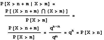
  The Geometric Random Variable, X, has the property that P[X>n+m | X>m] = P[X>n].  In words, if m tries have passed without a success, the probability that the first success occurs at least n trials later is doesn't depend on m.  This means that the the Geometric RV has no memory for what has occurred previously.  First an expression for P[X>n] is found: 

  

  Then 

  
  

  • Mean and Variance

    • Mean or Expected Value

      E[X] = 1 p + 2 pq + 3 pq² + 4 pq³ + ... = p(1 + 2q + 3q² + 4q³ + ...)

          = p(q + q² + q³ + q⁴ + ...)' = p (q/(1-q))' = p (((1-q)q' - q(1-q)')/(1-q)² )=

          p (((1-q) - q(-1))/(1-q)²) = p (1/(1-q)²) = p (1/p²) = 1/p
      
      

    • Variance

    E[X(X-1)] =  2 pq + 6 pq² + 12 pq³ + ... = p( 2 q + 6 q² + 12 q³ + ... )

        = p( q² + 2q³ + 3q⁴ + ...)' = p (q²(1+2q+3q²+...))' = p (q²(q+q²+q³+...)')') =

        p (q²(q/(1-q))')') = -2q/(1-q)³.  So E[X²]-E[X] = E[X²] - (1/p) = -2q/(1-q)³.  
    
     Then 
        Var[X] = E[X²] - E[X]² = (1/p) + 2q/(1-q)³ - (1/p)² = q/p²

To Top

• Properties of a Negative Binomial Random Variable with Parameters r and p

  • Definition

  1. An experiment is performed with the property that each performance of the experiment can result in a success, S, or failure, F with P[S] = p and P[F] = 1-p = q.  
  
  2. Each performance of the experiment is independent of all other performances.  
  
  3. The Negative Binomial Random Variable, X, with parameters r and p is the trial number of the rth success in the experiment. 
  

  • Simulation

  A Negative Binomial RV, X, with parameters r and p can be simulated as follows.  Generate random numbers between 0 and 1--after each number is generated check whether it is between 0 and p.  Keep a count of the number of random numbers generated, and the number that fall between 0 and p.  The trial number on which the rth number falling between 0 and p occurs is the value of X.
  
  Another way to simulate this random variable is to  place pieces of paper in a box--proportion p of the pieces of paper have 1's written on them, and the other pieces have nothing written on them.  Draw slips of paper replacing each one before drawing the next.  Let X=draw number at which the rth paper with a 1 is drawn.
  
  A simulation of a negative binomial random variable is found pressing the red die in front of Exercise 3 at this link.  

  • Probability Distribution (pdf)

  In developing the probability distribution of a negative binomial note that the pdf gives the probability of the rth success occurring at trial number k.  This means that in the preceding k-1 trials there must be r-1 successes.  The next statement shows this.

              p(k) = P[X=k] = _k-1C_r-1 p^r-1q^k-r p = _k-1C_r-1 p^r q^k-r for k=r, r+1, r+2, ... 
  
              p(k) = 0 for any other real k.

  As with any random variable the probabilities must sum to 1.  To show that the probabilities for the negative binomial sum to 1, a power series expansion that you might have seen in calculus can be used.  The power series for (1-q)^-r expanded about 0 is 

  
  

  If you sum the first few terms of the negative binomial pdf from above, you get p^r times the sum of terms shown above.  But the sum of terms shown above equals (1-q)^-r.  The sum of probabilities for the negative binomial with parameters r and p is p^r (1-q)^-r = p^r (p)^-r = 1.  

  • Mean and Variance

  To find the mean and variance of the the negative binomial use the relationship between the geometric and the negative binomial random variable.  Let X₁ be the trial number of the first success.  Let X₂ be the trial number of the second success (beginning the count on the trial immediately following the first success), let X₃ be the trial number of the third success (beginning the count on the trial immediately following the second success), etc.  X_r is the trial number of the rth success beginning the count on the trial immediately after the r-1st success.  Then the trial number of the rth success is X = X₁ + X₂ + X₃ + ... + X_n where X_i is a Geometric RV with parameter p.

  • Mean

  E[X] = E[X₁ + X₂ + X₃ + ... + X_r] = E[X₁] + E[X₂] + E[X₃] + ... + E[X_r] = 
                      1/p + 1/p + 1/p + ... + p = r p
  
  
  

  • Variance

  Var[X] = Var[X₁ + X₂ + X₃ + ... + X_r] = 
                          Var[X₁] + Var[X₂] + Var[X₃] + ... + Var[X_r] = 
                          q/p² + q/p² + q/p² + ... + q/p² = r q/p²

To Top

• Properties of a Poisson Random Variable with Parameter m

  • Definition

  A Poisson Random Variable with parameter m can be thought of as the limit of a binomial distribution distribution with parameters n and p as n approaches infinity and p approaches 0 in such a way that np = m.

  For example, suppose that you perform 10 independent Bernoulli trials with success parameter 0.2 and let Binomial RV X with parameters n and p equal the number of successes in the 10 trials.  X has mean np = 10 0.3 = 3.  Next, perform 100 independent Bernoulli trials with p=0.03.  If X is the number of successes, X has mean np = 100 0.03 = 3.  If you performed 1000 independent Bernoulli trials with p=0.003, the X has mean np = 1000 0.003 = 3.  The distribution that is the limit of these binomials is the Poisson Distribution.

  Parameter m is the average number of occurrences of the event of interest in a time or space interval.  Suppose you are counting telephone calls in 10 minute blocks of time.  If, on average, there are 3 phone calls per 10 minute interval, 3 is the value of m in the Poisson distribution.  The Poisson distribution gives the probabilities of various numbers of phone calls in a 10 minute interval.  There could be 0, or 1, or 2, or 3, or ... calls so the Poisson RV can take any of the values 0, 1, 2, ... .

  • Simulation

  The definition of the Poisson RV with parameter m indicates how it might be simulated.  Take n large and p small so that np = m and simulate a Binomial RV with parameters n and p.

  You can find a simulation of a Poisson Random Variable by clicking the red die in front of Exercise 3 at this link.
  
  

  • Probability Distribution (pdf) 

  The probability distribution is found by taking the limit of the binomial as n approaches infinity and p approaches 0 so that np = m or p=m/n.  In the binomial probability formula for k successes, p is replaced by m/n and the limit is found as n approaches infinity.  Thus, if k is 0 or any positive integer,

  

  In the last line, the limit of (1-(m/n))ⁿ as n approaches infinity is equal to e^-m.  This is a result that you have seen in in one of your calculus classes.

  In order to show that the last formula is a probability density function, the sum of P[X=k] for k=0, 1, 2, ... must equal 1.  To show this, you need to use another result from calculus, the power series expansion of e^x.  It is

  

  Then 

  

  using the expansion of e^x.

  • Mean and Variance

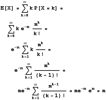
    • Mean
      
      
      

• Variance

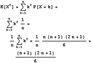
Var[X] = E[X²] - E[X]² = E[X²] - m² and E[X²] is computed in the next display.

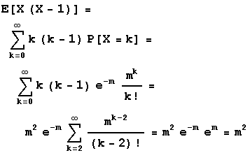
Now E[X(X-1)] = E[X²] - E[X] = m² or E[X²] = E[X] + m²  = m + m².  Then Var[X] = E[X²] - m² = m + m² - m² = m

To Top

• Properties of a Hypergeometric Random Variable with Parameters N, A, and n

  • Definition

  The Hypergeometric Random Variable with parameters N, A, and n is the count of the number of green balls in n draws without replacement taken from a container that holds N balls, A of which are green (think of the green balls as successes), and N-A are white (think of the white balls as failures).  

  • Simulation

  The Hypergeometric Random Variable with parameters N, A, and n can be simulated by placing N balls in a container with A of them colored green and the rest colored white.  Pick n balls without replacement and count the number of green balls picked.  This number is the value of the Hypergeometric RV with parameters N, A, and n.

  The Hypergeometric can be simulated on a computer by having the computer generate a random permutation of the integers 1 through N.  Consider integers 1 through A as the 'green balls' and the remaining integers as the 'white balls.'  After the random permutation of integers 1 through N is made, let the sample be the balls in positions 1 through n--the number of 'green balls' among them is the value of the Hypergeometric RV.

  You can find a simulation of the Hypergeometric RV as well as a comparison with the Binomial RV by following this link and pressing the red die in front of exercise 4.

  • Probability Distribution (pdf): 

  

  The probabilities must sum to 1 when summed over all possible values of k.  However, the following identity involving binomial coefficients can be shown:

  

  Dividing both sides of the last equality by the right hand side shows that the hypergeometric density function sums to 1.

  • Mean and Variance

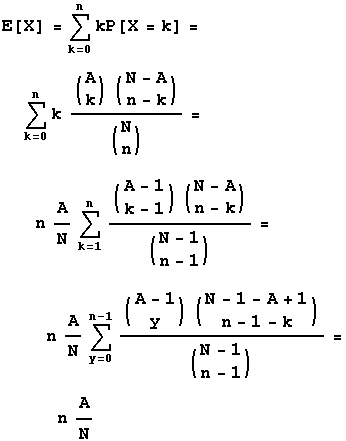
    • Mean
      
      

      

      
      

    • Variance

  The variance of the hypergeometric is computed by first finding E[X(X-1)].  This is n(n-1)[A(A-1)/(N(N-1))].  Then 

   

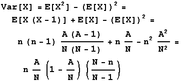
  Recall that the formula for the mean of a binomial is np and the variance of the binomial is npq.  If you think of A/N as p, the mean of a hypergeometric is much like the mean of the binomial.  The variance of the hypergeometric is of the form np(1-p)(N-n)/(N-1)=npq(N-n)/(N-1).  The extra term in the variance formula is called the 'finite population correction'.

To Top

• Properties of a Discrete Uniform Random Variable on the Integers 1, 2, ..., n

  • Definition

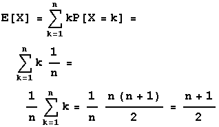
  A Discrete Uniform Random Variable on 1,2,3,...,n can assume any of these values with equal probability.  Since there are n values the probability of any value is 1/n.
  
  
  

  • Simulation

  A Discrete Uniform on 1,2,...,n can be simulated on the computer by dividing the interval [0,1] into n equal intervals [0,1/n), [1/n,2/n),...,[(n-1)/n,1].  Then generate a random number.  If the random number falls into the first subinterval, the Discrete Random Variable has value 1, if it falls into the 2nd subinterval, the RV has value 2, etc.

  It can be simulated by putting pieces of paper numbered from 1 through n in a hat and drawing a piece of paper.  The number on the piece of paper is the value of the Discrete Uniform RV.
  
   

  • Probability Distribution (pdf)

  P[X=k]=1/n if k=1,2,3,...,n and P[X=k]=0 for all other real numbers.

  It is easy to see that the probabilities sum to 1.
  
  

  • Mean and Variance
    

    • Mean
      
      

    • Variance

Then

To Top