Sampling Distributions
| Sampling Distribution of Sample Means |
| Normal Approximation to Binomial |
| Sampling Distribution of Sample Variance |
-
Introduction and Definitions
-
Introduction
At the beginning of this course you were introduced to populations, samples, and sampling from a population. It was stated that samples were to be used to make inferences about populations. You then learned to describe populations and samples graphically (histograms, boxplots, etc.) and numerically (means, medians, standard deviation, etc.). Next, you were introduced to concepts in probability, and you learned to apply these probability concepts to random variables. Finally, in the chapters leading up to sampling distributions, you were introduced to certain discrete (binomial, geometric, etc.) and continuous (normal, exponential, and uniform) random variables.
In this section on sampling distributions these ideas are combined into a method that can be used to make inferences about a population based on a random sample taken from the population.
This link takes you to a web page from Canada that expands on the concepts described in the previous paragraph.
-
Parameters and Statistics
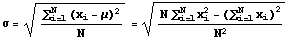
A population can be described numerically by its mean, standard deviation, median, and in many other numeric ways. When such a number is computed for a population, it is called a parameter of the population. Two parameters of populations that will be needed here are the population mean and population standard deviation. The formulas and symbols used to represent them are shown next, first the population mean and then the population standard deviation. Elements of the population are denoted by x1, x2, ... , xN.

A sample can be described numerically in the same way as a population. However, the numeric quantities that describe a sample are called statistics. Two statistics to be used here are the sample mean and sample standard deviation. The formulas and symbols for the sample mean and sample standard deviation statistics are shown next. Again, the first formula is for the sample mean and the second is for the sample standard deviation. The elements of a sample of size n taken from the population of size N are denoted by x1, x2, ... , xn.

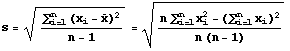
Notice that the formulas for the mean of a population and the mean of a sample are the same (except for the size of the population, N, and size of the sample, n). However, the formulas for standard deviation are different. The divisor is N in the formula for population standard deviation while it is n-1 for the sample standard deviation. This slightly different formula is used because it gives a better estimate of the population standard deviation (in statistical terminology dividing by n-1 makes the sample standard deviation an unbiased estimator for the population standard deviation).
-
Sampling Distributions of Statistics
The sampling distribution of a statistic is the distribution of that statistic for all possible samples of fixed size, say n, taken from the population. For example, if the population consists of numbers 1,2,3,4,5, and 6, there are 36 samples of size 2 when sampling with replacement. If the sample mean is computed for each of these 36 samples, the distribution of these 36 sample means is the sampling distribution of sample means for samples of size 2 taken with replacement from the population 1,2,3,4,5, and 6. Likewise, you could compute the sample standard deviation for each of the 36 samples. The distribution of these 36 sample standard deviations is the sampling distribution of sample standard deviations for all samples of size 2 taken with replacement from the given population.
The sampling distributions of these and other statistics need to be studied in order to develop principles for making inferences about a population based on a random sample from that population. In practice, a single sample of a certain size, n, is usually selected, and population inferences are made from this single sample. However, in order to see what can be inferred about the population from a single sample, we must first look at all, or, at least, a large number of samples of size n taken from the given population. For each sample the statistic of interest is computed and the distribution of all or a large number of these statistics is determined. From this sampling distribution, principles of inference are developed. In this presentation the sampling distributions of sample means and sample standard deviations are introduced.
-
To Top
The sampling distribution of a sample mean is the distribution of all sample means for samples of a fixed size, say n, taken from some population, usually without replacement, although for mathematical convenience, sampling with replacement is investigated first. Also, in most cases the population has many members (i.e., the population size, N, is large). The size of the population is often the major reason for using sampling--if the population were very small, you could survey the entire population and make statements based on the entire population. For convenience, a very small population is used in the next example.
In this first example, the population consists of the numbers 1,2,3,4,5, and 6. The 36 random samples of size 2 taken with replacement from this population are shown in the next table. Also shown are the sample means, sample standard deviations (stdev), and sample variances (var) for each sample. This sampling situation can be simulated by tossing a pair of fair dice--for convenience, suppose one die is colored green and the other is the normal white color. The number on the white die is shown in the column at the left of the table, and the number on the green die is shown across the top of the table.
1 2 3 4 5 6 1 1,1
mean=1
stdev=0
var=01,2
mean=1.5
stdev=0.71
var=0.5041,3
mean=2
stdev=1.41
var=1.991,4
mean=2.5
stdev=2.12
var=4.491,5
mean=3
stdev=2.83
var=8.011,6
mean=3.5
stdev=3.54
var=12.532 2,1
mean=1.5
stdev=0.71
var=0.5042,2
mean=2
stdev=0
var=02,3
mean=2.5
stdev=0.71
var=0.5042,4
mean=3
stdev=1.41
var=1.992,5
mean=3.5
stdev=2.12
var=4.492,6
mean=4
stdev=2.83
var=8.013 3,1
mean=2
stdev=1.41
var=1.993,2
mean=2.5
stdev=0.71
var=0.5043,3
mean=3
stdev=0
var=03,4
mean=3.5
stdev=0.71
var=0.5043,5
mean=4
stdev=1.41
var=1.993,6
mean=4.5
stdev=2.12
var=4.494 4,1
mean=2.5
stdev=2.12
var=4.494,2
mean=3
stdev=1.41
var=1.994,3
mean=3.5
stdev=0.71
var=0.5044,4
mean=4
stdev=0
var=04,5
mean=4.5
stdev=0.71
var=0.5044,6
mean=5
stdev=1.41
var=1.995 5,1
mean=3
stdev=2.83
var=8.015,2
mean=3.5
stdev=2.12
var=4.495,3
mean=5
stdev=1.41
var=1.995,4
mean=4.5
stdev=0.71
var=0.5045,5
mean=5
stdev=0
var=05,6
mean=5.5
stdev=0.71
var=0.5046 6,1
mean=3.5
stdev=3.54
var=12.536,2
mean=4
stdev=2.83
var=8.016,3
mean=4.5
stdev=2.12
var=4.496,4
mean=5
stdev=1.41
var=1.996,5
mean=5.5
stdev=0.71
var=0.5046,6
mean=6
stdev=0
var=0The collection of 36 sample means constitutes the sampling distribution of sample means for samples of size 2 taken with replacement from the population 1,2,3,4,5, and 6. Since each one of these 36 sample means occurs with equal probability, the probability distribution of the sample means can easily be found and is displayed in the next table. Later, the probability distribution of sample standard deviations will be studied.
Sample Mean 1 1.5 2 2.5 3 3.5 4 4.5 5 5.5 6 Probability 1/36 2/36 3/36 4/36 5/36 6/36 5/36 4/36 3/36 2/36 1/36 The mean of this sampling distribution of sample means for samples of size 2 equals (1)(1/36)+(1.5)(2/36)+(2)(3/36)+...+(6)(1/36) = 3.5.
The variance of this distribution is E[X2]-(E[X])2. E[X] was just computed and equals 3.5. E[X2]=(12)(1/36)+(1.52)(2/36)+(22)(3/36)+...+(62)(1/36) = 13.71. Then Var[X]=13.71-(3.52)=1.458. The standard deviation is the square root of the variance, or 1.21.
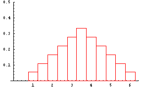
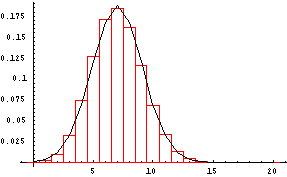
The graph of the sampling distribution of sample means is shown next.
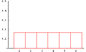
This probability distribution doesn't look like the distribution of the population from which the samples were selected. The distribution of the population is shown in the next table followed by a graph of that distribution.
Number 1 2 3 4 5 6 Probability 1/6 1/6 1/6 1/6 1/6 1/6 The mean or expected value of the population is (1)(1/6)+(2)(1/6)+(3)(1/6)+(4)(1/6)+(5)(1/6)+(6)(1/6)=3.5.
The variance of this distribution is E[X2]-(E[X])2. E[X] was just computed and equals 3.5. E[X2]=(12)(1/6)+(22)(1/6)+(32)(1/6)+(42)(1/6)+(52)(1/6)+(62)(1/6)=15.17. Then Var[X]=15.17-3.52 =2.92, so the standard deviation is the square root of 2.92, or 1.71.
The graph of this population probability distribution is shown below.
Looking at the graphs of these two probability distributions and their underlying probability tables, what are the relationships between them? First, the means are equal, secondly, the standard deviation of the sample distribution is smaller than the standard deviation of the population. Finally, what about the graph shapes? In order to answer this question, take a look at the next link.
Follow this link to reach a page that shows a simulation of the distribution of sample means and other statistics for the dice experiment. When you reach the page, press the red die in front of exercise 2 to see the dice experiment simulation. Use this simulation to investigate the theoretical probability distribution of sample means (blue histogram) for samples of size n as n is increased.
Perhaps the symmetry and uniformity of the population is reason that the distribution of sample means looks more like a normal distribution as the sample size increases. To see a Java simulation that shows the distribution of sampling means approaches a normal distribution regardless of population shape, follow this link. When the Java applet opens, you can choose the shape of the population. The simulation shows what happens when a large number, rather than all, samples of a certain size are taken.
The main points demonstrated in these examples:
The mean of the distribution of sample means equals the mean of the population, or symbolically,
The standard deviation of the distribution of sample means for samples of size n equals the standard deviation of the population divided by the sample size, or symbolically,
Or, equivalently, in terms of variance,
Central limit theorem: The sampling distribution of sample means is approximately normally distributed. The approximation is better for larger values of n. If the population has a normal distribution, the sampling distribution of sample means is exactly normally distributed.


To Top
The normal approximation to the binomial distribution was a more useful computational aid in the days before the powerful computers and hand-held calculators that are available today. It is introduced here as an application of the central limit theorem. Recall that a binomial random variable, Y, with parameters n and p is the count of successes in n independent experiments, each of which can result in a success with probability p and failure with probability q=1-p. Recall that defining X1=1 if the 1st experiment is a success and 0 otherwise, X2=1 if the 2nd experiment is a success and 0 otherwise, ..., and Xn=1 if the nth experiment is a success and 0 otherwise, Y=X1+X2+...+Xn. Each of these random variables has a Bernoulli distribution with parameter p--this implies that each of the X's has mean p and variance pq. Y has a mean of np and variance of npq. From the result noted above, if n is 'large,' Y/n will have an approximate normal distribution with mean of Y/n=E[Y/n]=(1/n)E[Y]=np/n=p and variance of Y/n=Var[Y/n]=(1/n2)Var[Y]= npq/n2=pq/n. It is then easy to believe that Y=n(Y/n) should have an approximate normal distribution with mean np and variance npq.
The next graph shows the pdf of a binomial random variable with n=20 and p=0.35 together with an approximating normal curve. The mean is 20(0.35)=7 and variance is 20(0.35)(0.65)=4.55 so standard deviation=2.13. A rule of thumb says that whenever np and n(1-p) are both greater than 5, the normal approximation to the binomial can be used.
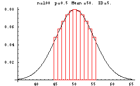
Suppose you are asked to compute the probability of getting exactly 50 heads in 100 tosses of a fair coin. The number of heads in 100 tosses is a binomial random variable with parameters 100 and p=1/2. P[50 Heads]=100C50(1/2)50(1/2)50. You can find the value of this on most calculators but this computation caused an overflow or underflow on many calculators that were in use 10 years ago. Since 100(1/2)=50>5, the normal approximation to the binomial can be used. The graph of the binomial is shown in red with the probability of 50 heads equal to the area of the red bar centered at 50.
The normal curve provides a good approximation to the binomial. To approximate the probability of 50 heads, find the area under the normal curve between the left and right hand sides of the red bar centered at 50. To do this you must find the z-values at 49.5 and 50.5. They are (49.5-50)/5=-0.1 and (50.5-50)/5=0.1. You can use the normal table to find that the approximate probability of 50 heads is 0.0797. Using the formula for binomial probabilities, you would get 0.0796.
In the experiment of tossing a fair coin 100 times, what is the probability that the number of heads will be between 48 and 54, inclusive. To find this exactly you would need to add the probabilities of 48, 49, 50, 51, 52, 53, and 54 heads together. In the graph shown above this would be equivalent to finding the sum of the areas of the red bars beginning with the bar centered at 48 and ending with the bar centered at 54. Using the normal approximation, you could find the z-score at the left side of the smallest bar, that is at 47.5, and the z-score at the right side of the largest bar, that is at 54.5, and then use the normal table to find the area between. If you carry this out, you get a normal approximation probability of 0.5074. If you used the binomial formula, you would find the exact probability is 0.5072.
The link shown in the next sentence provides comparisons of exact binomial probabilities and the normal approximations. A link to the normal approximation to a binomial random variable is found here.
To Top
From the above table showing all samples of size 2 with replacement taken from the population 1,2,3,4,5, and 6, you can construct the sampling distribution of the sample variance. Simply square each of the standard deviations and pair the standard deviations with their probabilities as shown in the next table.
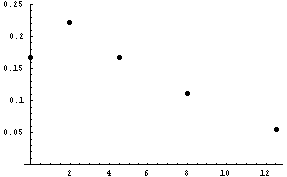
| Sample Variance | 0 | 0.504 | 1.99 | 4.49 | 8.01 | 12.53 |
| Probability | 6/36 | 10/36 | 8/36 | 6/36 | 4/36 | 2/36 |
The expected value of this sampling distribution is (0)(6/36) + (0.504)(10/36)+(1.99)(8/36)+(4.49)(6/36)+(8.01)(4/36)+(12.53)(2/36)=2.92. This is the variance of the population.
The variance of this sampling distribution can be computed by finding the expected value of the square of the sample variance and subtracting the square of 2.92. The variance is 11.65.
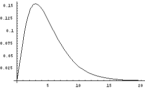
The probability distribution for the sample variances is shown next. This graph shows no negative values on the horizontal axis. This is always true for variances because variances can't be negative. Secondly, the graph does not have the symmetric look of the graph of sample means. In fact, the graph of the sample variance distribution will always be skewed to the right.
From this sampling distribution of sample variances, the only conclusion that can be made is that the expected or mean value of sample variances is the population variance. You can follow this link to see a simulation of sample variances when sampling from any type of population. In order to make further statements about the sampling distribution of sample variances, the population from which samples are selected must have a normal distribution. In that case, it can be shown that the sampling distribution of sample variances has a special form called a chi-square distribution with one parameter, the parameter being the sample size minus one (n-1). This parameter is called the degrees of freedom of the chi-square distribution. The next graph shows the probability density function of a chi-square distribution with 5 degrees of freedom. Notice that it is skewed to the right.
In general, when samples of size n are taken from a normal distribution with variance
, the sampling distribution of the
has a chi-square distribution with n-1 degrees of freedom.